How to Use Excel Pivot Tables to Organize Data

excel pivot tables are a feature that you should learn how to use. Instead of analyzing countless spreadsheet records, these tables can aggregate your information and show a new perspective in a few clicks. You can also move columns to rows or vice versa. The problem is people believe creating a pivot table is difficult to learn. Grab a seat and we’ll guide you through a short tutorial so you can start data crunching. (Check Resources section at bottom for example worksheet.)

What is an Excel Pivot Table?

You might think of a pivot table as a user-created summary table of your original spreadsheet. You create the table by defining which fields to view and how the information should be displayed. Based on your field selections, Excel organizes the data so you see a different view of your data.

As example, I’ve uploaded a sample spreadsheet of 4000 fictitious people, which includes the following data fields:

• Voter ID
• Party Affiliation
• Their precinct
• Age group
• When they last voted
• Years they’ve been registered
• Ballot status

Looking at the first 20 voter records, you can see the content is boring. In this format, the key question it answers is how many voters exist in all the precincts.

Using Excel pivot tables, you can organize and group the same data in ways that start to answer questions such as:

• What is the party breakdown by precinct?
• Do voters use permanent absentee ballots?
• Which precincts have the most Democrats?
• How many voter pamphlets do I need for Precinct 2416?
• Do 18-21 year olds vote?

Excel pivot tables allow you to group the spreadsheet or external data source by any of your data fields. The screen snap below shows a count of voters by party by precinct.

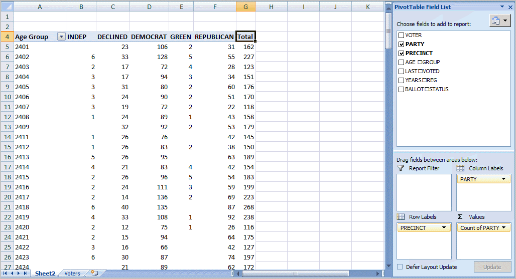
Using a pivot table, I can continue to slice the information by selecting more fields from the PivotTable Field List. For example, I can take the same data and segment by voter age group.

Understanding the Table Structures

In the screen snap above, I’ve labeled the main areas of the pivot table.

1. PivotTable Field List – this section in the top right displays the fields in your spreadsheet. You may check a field or drag it to a quadrant in the lower part.
2. The lower right quadrants – this area defines where and how the data shows on your pivot table. You can have a field show in either a column or row. You may also indicate if the information should be counted, summed, averaged, filtered and so on.
3. The red outlined area to the left is the result of your selections from (1) and (2). You’ll see that the only difference I made in the last pivot table was to drag the AGE GROUP field underneath the PRECINCT field in the Row Labels quadrant.

How to Create an Excel Pivot Table

There are several ways to build a pivot table. Excel has logic that knows the field type and will try to place it in the correct row or column if you check the box. For example, numeric data such as Precinct counts tends to appear to the right in columns. Textual data, such as Party would appear in rows.

While you can simply check fields to display and let Excel build your pivot table, I prefer to use the “drag and drop” method. This is partly because I like to visualize my data in columns and rows. I think it may also be easier if you have fields, which can appear to be numbers like a precinct value.

1. Open your original spreadsheet and remove any blank rows or columns.
2. Make sure each column has a heading, as it will be carried over to the Field List.
3. Make sure your cells are properly formatted for their data type.
4. Highlight your data range
5. Click the Insert tab.
6. Select the PivotTable button from the Tables group.
7. Select PivotTable from the list.

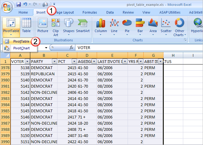
The Create PivotTable dialog appears.

8. Double-check your Table/Range: value.
9. Select the radio button for New Worksheet.
10. Click OK.

A new worksheet opens with a blank pivot table. You’ll see that the fields from our source spreadsheet were carried over to the PivotTable Field List.

11. Drag an item such as PRECINCT from the PivotTable Field List down to the Row Labels quadrant. The left side of your Excel spreadsheet should show a row for each precinct value. You should also see a check mark appear next to PRECINCT.

12. The next step is to ask what you would like to know about each precinct. I’ll drag the PARTY field from the PivotTable Field List to the Column Labels quadrant. This will give an extra column for each party. Note that you won’t see any numerical data.

13. To see the count for each party, I need to drag the same field to the Valuesquadrant. In this case, Excel determines I want a Count of PARTY. I could double-click the entry and choose another Field Setting. Excel has also added Grand Totals.

Additional Groupings and Options

As you build your Excel pivot table, you’ll probably think of more ways to group the information. For example, you might want to know the Age Range of voters by Precinct by Party. In this case, I would drag the AGE GROUP column from the PivotTable Field List down below the PRECINCT value in Row Labels.

Each age group is broken out and indented by precinct. At this stage, you might also be thinking of usability. As with a regular spreadsheet, you may manipulate the fields. For example, you might want to rename “Grand Total” to “Total” or even collapse the age values for one or more precincts. You can also hide or show rows and columns. These features work the same way as a regular spreadsheet.

One area that is different is the pivot table has its own options. You can use these options by right-clicking a cell within and selecting PivotTable Options… For example, you might only want Grand Totals for columns and not rows.

There are also ways to filter the data using the controls next to Row Labels or Column labels on the pivot table. You may also drag fields to the Report Filter quadrant.

Troubleshooting Excel Pivot Tables

You might encounter several “gotchas” with this example file or another spreadsheet. Sometimes when you move around your pivot table the PivotTable Field Listdisappears. To get it back, click any cell with a value.

You can also move or “pivot” your data by right clicking a data field on the table and selecting the “Move” menu. From here, you can move a column to a row or even change the position. An example of this might be the values for “LAST VOTED” since Excel will sort by the month first. You might prefer to move the data so the election dates are in a chronological order.

I prefer not adding fields to a pivot table. I think it’s easier to add the fields first to your source spreadsheet. The reason is you might get items out of sync if you move data unless you make them a calculated field.

Excel pivot tables may not make the election data exciting, but it can make the analysis easier. Without these tables, you’d probably spend more time filtering, sorting and subtotaling. The other benefit is that it’s easy to start over by deselecting fields or moving them to another place. Feel free to download the tutorial spreadsheet below and play with the data. This may be the only time you’re allowed to manipulate election data.

Pivot Tables

Pivot tables are one of  excel is most powerful features. A pivot table allows you to extract the significance from a large, detailed data set.

Our data set consists of 214 rows and 6 fields. Order ID, Product, Category, Amount, Date and Country.

1. Click any single cell inside the data set.

2. On the Insert tab, click PivotTable.

The following dialog box appears. Excel automatically selects the data for you. The default location for a new pivot table is New Worksheet.

3. Click OK.

Drag fields

The PivotTable field list appears. To get the total amount exported of each product, drag the following fields to the different areas.

1. Product Field to the Row Labels area.

2. Amount Field to the Values area.

3. Country Field to the Report Filter area.

Below you can find the pivot table. Bananas are our main export product. That's how easy pivot tables can be!

Click any cell inside the Total column.2. The PivotTable Tools contextual tab activates. On the Options tab, click the Sort Largest to Smallest button (ZA).

Result.

Filter

Because we added the Country field to the Report Filter area, we can filter this pivot table by Country. For example, which products do we export the most to France?

1. Click the filter drop-down and select France.

Result. Apples are our main export product to France.

Note: you can use the standard filter (triangle next to Product) to only show the totals of specific products.

Change Summary Calculation

By default, Excel summarizes your data by either summing or counting the items. To change the type of calculation that you want to use, execute the following steps.

1. Click any cell inside the Total column.

2. Right click and click on Value Field Settings...

3. Choose the type of calculation you want to use. For example, click Count.

4. Click OK.

Result. 16 out of the 28 orders to France were 'Apple' orders.

Two-dimensional Pivot Table

If you drag a field to the Row Labels area and Column Labels area, you can create a two-dimensional pivot table. For example, to get the total amount exported to each country, of each product, drag the following fields to the different areas.

1. Country Field to the Row Labels area.

2. Product Field to the Column Labels area.

3. Amount Field to the Values area.

4. Category Field to the Report Filter area.

Below you can find the two-dimensional pivot table.

To easily compare these numbers, create a pivot chart and apply a filter. Maybe this is one step too far for you at this stage, but it shows you one of the many other powerful pivot table features Excel has to offer.

Excel 2010

Saving workbooks

Video: Saving Workbooks in Excel 2010

When you create a new workbook in Excel, you'll need to know how to save it to access and edit it later. excel allows you to save your documents in several ways.

Optional: You can download this example for extra practice.

To use the Save As command:

Save As allows you to choose a name and location for your workbook. Use it if you are saving a workbook for the first time or if you want to save a different version of a workbook while keeping the original.

1. Click the File tab.
2. Select Save As.
   
3. The Save As dialog box will appear. Select the location where you want to save the workbook.
4. Enter a name for the workbook, then click Save.
   

If you are using Windows 7, you will most likely want to save files to your Documents library. For other versions of Windows, you will most likely want to save files to the My Documents folder. For more information, check out our lessons on Windows 7 and Windows XP.

To use the Save command:

1. Click the Save command on the Quick Access toolbar.
   
2. The workbook will be saved in its current location with the same file name.

If you are saving for the first time and select Save, the Save As dialog box will appear.

To use AutoRecover:

Excel automatically saves your workbooks to a temporary folder while you're working on them. If you forget to save your changes or if Excel crashes, you can recover the autosaved file.

1. Open a workbook that was previously closed without saving.
2. In Backstage view, click Info.
3. If there are autosaved versions of your workbook, they will appear under Versions. Click the file to open it.
   
4. A yellow caution note will appear on the Ribbon of the workbook. To restore this version of the workbook, click Restore, then click OK.
   

By default, Excel autosaves every 10 minutes. If you are editing a workbook for less than 10 minutes, Excel may not create an autosaved version.

If you do not see the file you're looking for—or if you're looking for an autosaved version of a file that has no previously saved versions—you can browse all autosaved files by clicking the Manage Versions button and selecting Recover Unsaved Workbooks from the drop-down menu.

An Excel Template for Every Occasion

Getting the best out of excel can sometimes be daunting. Known for its functions, formulas, and data analysis capacities, it might leave you wondering how you can use Excel as a practical productivity tool in your life, without the steep learning curve.

You can streamline your organization skills using the massive range of Excel templates: money, budgeting, payslips, project management, and much more can be efficiently managed, freeing up time for…well, more awesome things.

You can download well balanced, auto-updating Excel templates that you, or anyone you share your work with, can use straight away. It’ll be EXCEL-LENT!

Budget Templates

I’ve included a few budget templates as they come in numerous flavors. I’m still relatively new to budgeting. Having been quite the carefree student, I suddenly found myself a family-man, so learning to account for each penny quickly became a must. I have some of these Excel budget templates to thank.

Family Budget Planner

I went from party-animal student, to student with partner-expecting-child, to terrified-student-father in a matter of months (let’s assume it was 9…). This little template helped me no end, and it’ll certainly help you, too. It’s thorough, well planned, and has a number of savings and planning functions.

It isn’t limited to Excel either. Once downloaded, this template works perfectly well in Open Office, LibreOffice, and Google Sheets – all perfect for really squeezing that budget, if propriety software has its own column.

Money Management

A big part of understanding your budget is effective money management: where it’s coming from, where it’s going, your debtors, your creditors, and everything else you can think of. When you have so many different sources coming into and out of multiple checking accounts, plus a mortgage, plus your business accounts, you can quickly lose track of incomings and outgoings. Unless you use a handy spreadsheet like this:

Event Budget

I’m planning my wedding at this very moment. Huhrah /s. At the moment, the immense excitement is being seriously overawed by the minute finance management my partner and I seem to spend most of our waking time talking about. We’ve kept right on top of things using a dedicated Event Budget planner – and so far it’s helped us come in way under-budget.

We’ve used it for our wedding planning, but you can use it for your fundraiser, your social event, or if you’re throwing a big ol’ shindig.

Fundraiser Thermometer Template

Visualizing your progress toward a finance goal can provide the extra impetus to get you over the line – and further! Some people are just visually inspired, whilst others find visualizing a numerical amount makes it easier to interpret. Give this one a look:

It isn’t the flashiest, but you can add On Track Targets, calculate donations for specific period, or donations for a single day.

Maintenance Schedule Template

Home ownership comes with many additional tasks, aside from the massive repayments. You can no longer call your landlady and cry down the phone because the gas boiler is broken and you really, really wanted a hot bath.

No, you’ll need to keep up with regular home maintenance or else it’ll literally start falling apart. Keep abreast of what needs doing, and when, with a handy home maintenance template. In this case, I’ve used an inbuilt Excel template as it has everything I need, but you can search for ones that suit your home repair schedule.

Database Template

Much like the budget templates, I’ve included a few database templates as they come in so many flavors. You might have to try a few before you find one that fits your data processing requirements, be that home or business use.

CRM

You can use Excel as an effective CRM system for your business. Streamline communications with existing and potential clientele to gain a competitive edge, using a free template. As they say, take care of the little things, and the big things will take care of themselves.

Inventory Management

Running a small business – or a large one – requires organization. If you’ve a warehouse full of stock, you need to keep track of each coming and going, ensuring that each day your database is updated. It doesn’t take Warren Buffet to understand stock management. This is an inbuilt Excel template, but there are plenty more available across the web.

Payroll Management

Managing your employees is essential – they’d be mighty disappointed if they realized all of their financials were written on a napkin, stashed underneath that snazzy Home Depot paperweight. Use a preformatted template to keep track of your employees – their total and hourly rates, their SS numbers, their over-time status, and 401(K) contributions.

Planning Templates

Are you a project manager? Or builder? Or simply work in an office, with deadlines? Let’s go further: do you actively plan aspects of your live to ensure there aren’t any massive blips? You’ll love these Excel planning templates.

Gantt Chart

A Gantt Chart template is essential for any project you are tasked with managing. Ever tried managing without one? I cannot fathom how you succeeded, if indeed you did. Gantt Charts are another excellent time visualization tool, helping you plan each aspect of your project in correlation. Use one – I guarantee it will help.

The best part is the automation. Add a detail, or edit the timeline, and your template will automatically update each correlating detail.

Continuous Monthly Calendar

I’ve only just started using a continuous monthly calendar, but it has quickly made a few differences to my work flow. Along with the budgeting, getting to grips with a real-life work flow following the many years of university was a challenge, but something I’ve steadily improved on over the years. Little tools like this can make all the difference if you’ve several different sources of work running concurrently, with smatterings of deadlines along with more work appearing.

Weekly, Bi-Weekly and Monthly Timesheets

Keep abreast of your hours worked. Even if you have a login system in the workplace, you should be tracking your hours. If there are any discrepancies or shortcomings in your paycheck, you’ve tracked each and every hour worked. It also helps you plan your incomings and outgoings a little better, and understand the value in time.

Other Planning Templates

It isn’t always about business. The inbuilt Excel templates feature gardening schedules for the green fingered, family meal planning for the waste conscious, and detailed family travel itineraries for those efficient fun-having parents. Scroll through the Excel template repository, or search using “Planning” to bring up a number of relevant results.

Excel Template Sources

If you want to continue your productivity drive, check out these Excel template sources:

• Spreadsheet123
• Vertex42
• Office Store
• Excel Templates
• Chandoo

Once you start managing more of your life with Excel templates, you’ll have so much time for other activities, you’ll have to design a new template to keep track of your new-found time-wealth. And hopefully some monetary wealth, too.

Do you use templates? What’s your favorite time-saver? Are you a meticulous planner? Let us know below!