How to correct a #VALUE! error

Applies To:  , excel Excel 2013 , Excel 2010 , Excel 2007 , Excel 2016... for Mac , Excel Starter

The most common reason for the #VALUE! error is that a formula is expecting numbers in a cell, but instead it finds spaces, text, or other characters.

Top solution - Try using functions instead of operators

Formulas with math operators like +, -, *, ^ and / may not be able to calculate cells that contain text or spaces. In this case, try using a function instead. Functions will often ignore text values and formulate everything as numbers, eliminating the #VALUE! error.

If you’re not sure what to do at this point or what kind of help you need, you can search for similar questions in the Excel Community Forum, or post one of your own.

If you want to move forward, then the following checklist provides troubleshooting steps to help you figure out what may have gone wrong in your formulas.

Finding where a formula is broken with the Evaluate Formula Wizard

If your formula is throwing a #VALUE! error, but you don't know where it is, you can use the Evaluate Formula Wizard. Select the cell with the error and goto Formulas > Evaluate Formula, and an interactive dialog will appear:

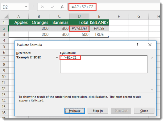
Each time you click the Evaluate button, Excel will step through the formula and calculate each part individually, then display the results. This won't fix your formula, but it can help you figure out where it's breaking, so you can go fix it. In this case the formula =A2+B2+C2 breaks because of a leading space in cell A2, but you can't see it. The Evaluate Formula Wizard does though and it shows that the value is =" "+B2+C2, where the " " indicates a blank space.

Check for hidden spaces inside cells

Sometimes cells look blank, when in fact they may have hidden spaces. Double-click a cell that your formula is referencing (or press F2), and check for spaces. In the following illustration, there are extra spaces to the left of cursor in cell A2.

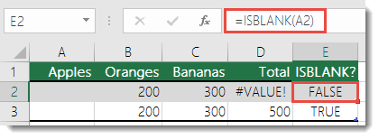
Try deleting the spaces, or select the cell and press Delete to see if the error goes away. If you have many rows to check, you can use the ISBLANK() function in an empty column to see if cells are truly blank or not. In the following illustration, cell A2 has a hidden space that you can’t see, and the ISBLANK function in E2 returns FALSE. Whereas A3 is truly blank and the ISBLANK function returns TRUE.

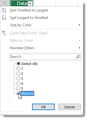
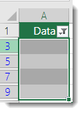
Tip: Use Auto Filter to mass delete blank cells. You can click Data > Filter and Filter for Blanks on the column with blanks (Auto Filter will see cells with leading spaces as blanks as well). Next, select the entire column and press CTRL+G (Goto) > Special > Visible Cells only, then press DELETE to clear everything.

Clean text using the CLEAN function

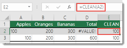
Sometimes when you import data from external sources, it can come into Excel with non-printing characters like ^ or '. Unfortunately, these characters can cause problems in formulas and it can be hard to delete them. However, you can use the CLEAN function to strip the characters out, and convert the values from text to numbers. You can then copy the CLEAN function range and paste just the cell values back over the original range. Here’s how: Select the CLEAN function range, and then press CTRL+C. Select the original cells and click Home > Paste > Paste Special > Values (or Alt > E > S > V for keyboard shortcuts for the PC - For MAC you can use  +OPTION + V > V > Enter).

Clean text using the TRIM function

Sometimes leading or trailing spaces can cause problems. Excel will generally try to remove these spaces in simple values. For example, it will remove spaces if you type “ 123”, but it might not be able to do the same with date values like “ 1/1/16”. In this case, you can use the TRIM function to remove those leading and trailing spaces, and then reference the converted TRIM value in your calculation, or use the Copy > Paste Special > Values method to replace the original values.

In this example, leading spaces in the date in A2 cause a #VALUE! error with =B2-A2. But by using =TRIM(A2), we can then use =B2-D2 to resolve the error.

Check if the formula is referencing cells that contain text

Right-click a cell that the formula is referencing, and then click Format Cells (or use CTRL+1). Make sure the format is not Text. Sometimes this is not practical for more than one cell, so if you have more than one to check, insert a new column and use the ISTEXT() function to see if the cells are formatted as text. In the example below “173 0” isn’t a valid number, so Excel will see it as text. This can often be the result of a typo. Note that ISTEXT won’t resolve the error, it will just tell you if text could be causing the issue.

Your workbook uses a data connection that isn't available

To fix this, restore the data connection, or consider importing the data if possible. This can happen a lot with distributed workbooks, where you might send a workbook to someone who doesn't have the data connection. In cases like this it can be a good idea to create a distribution copy where you copy an entire worksheet(s) and Paste > Special >Values, which will eliminate formulas and links.

Replace the #VALUE! error with something else

Sometimes you just want to replace the #VALUE error with something else like your own text, a zero or a blank cell. In this case you can add the IFERROR() function to your formula. IFERROR() will check to see if there’s an error, and if so, replace it with another value of your choice. If there isn’t an error, your original formula will be calculated. IFERROR will only work in Excel 2007 and later versions. For earlier versions you can use IF(ISERROR()).

Warning: IFERROR is a blanket error handler, meaning that it will suppress all errors, not just the #VALUE! error. It’s not advisable to use IFERROR until you are absolutely certain that your formula performs the way that you want. Otherwise, you won’t see potentially valuable error messages that might indicate you have a problem.

Here’s an example of a formula that has a #VALUE! error due to a leading space in cell D2:

And here’s the same example with IFERROR applied to replace #VALUE! with zero:

You could also use =IFERROR(C2-D2,””) to display nothing instead of 0, or even substitute your own text, like: =IFERROR(C2-D2,”Discount Error”).

Unfortunately, you can see that IFERROR doesn’t actually resolve the error, it simply hides it. So be certain that hiding the error is better than fixing it.